This paper is available on arxiv under CC 4.0 license.
Authors:
(1) Z. Jennings, Astrophysics Group, Keele University, Staffordshire, ST5 5BG, UK (E-mail: z.jennings@keele.ac.uk);
(2) J. Southworth, Astrophysics Group, Keele University, Staffordshire, ST5 5BG, UK;
(3) K. Pavlovski, Department of Physics, Faculty of Science, University of Zagreb, 10000 Zagreb, Croatia;
(4) T. Van Reeth, Institute of Astronomy, KU Leuven, Celestijnenlaan 200D, B-3001 Leuven, Belgium.
Table of Links
- Abstract and Intro
- Observation
- Orbital Ephemeris
- Radial Velocity Analysis
- Spectral Analysis
- Analysis of the Light Curve
- Physical Properties
- Asteroseismic Analysis
- Discussion
- Conclusion, Data Availability, Acknowledgments, and References
- Appendix A: Ephemeris Determination
- Appendix B: Iteratively Prewhitened Frequencies
- Appendix C: Detected Tidally Perturbed Pulsations
4 RADIAL VELOCITY ANALYSIS
The spectral range between 4400–4800 Å is a suitable region to carry out the RV extraction procedure because there are many wellresolved spectral lines and the region does not contain any wide Balmer lines. Thirteen échelle orders within this range were corrected for cosmic ray spikes by first resampling onto a homogeneous wavelength grid before using a median filter to smooth them, then resampling the orders back to the original grid and subtracting them from the observed spectrum (Blanco-Cuaresma et al. 2014a). Pixels where the residual deviated by a threshold percentage, typically between 5 and 10%, were masked and their values were corrected for using linear interpolation. The appropriate value for the threshold was investigated for each order individually based on visual inspections of resulting flagged pixels. The blaze signature was removed using the method of Xu et al. (2019), where alpha shape fitting (see, Edelsbrunner et al. 1983) combined with local polynomial regression is used to estimate the continuum without dividing out important spectral features.
Small errors in the continuum estimation are magnified where the blaze function approaches zero. Following Xu et al. (2019), a better estimation at the edges can be obtained by taking a weighted average in the overlapping regions and applying weights such that pixels further away from the edge within their own order are favoured. For this to be applied correctly, the orders were re-sampled onto grids with a common wavelength step so that the pixel averages were calculated for corresponding wavelength values between neighbouring orders. A useful result from the edge correction procedure is that neighbouring orders share a common edge and can be merged after truncating the orders in the centre of the overlapping regions. The following analysis was carried out after merging the 13 spectral orders with wavelengths between 4400-4800 Å using this process.
The pulsating eclipsing binary KIC 9851944
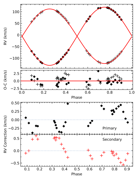
Our own implementation of the TODCOR two-dimensional cross-correlation algorithm (Zucker & Mazeh 1994) was used to extract the RVs. Systematic errors arise when using the cross-correlation technique to extract RVs because neighbouring peaks and sidelobes in the doubled-peaked CCF disturb each other, and this is related to blending between the spectral lines of the two components (Andersen 1975; Latham et al. 1996). The result is that the estimated RVs may be shifted relative to the true value, where the size and direction of the shift depends on the phase (see Fig.4), i.e, the relative Doppler shifts between the components (Latham et al. 1996).
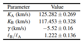
This systematic error can be minimised by correcting the RVs for this effect (e.g., Latham et al. 1996; Torres et al. 1997; Torres et al. 2000; Torres & Ribas 2002; Southworth & Clausen 2007). A preliminary orbit was obtained by making an initial fit to the RVs extracted using TODCOR. A synthetic SB2 model was then produced with orbital parameters corresponding to the initial fit by Doppler shifting and adding the template spectra weighted by their relative light contributions as estimated by the resulting value for ℓB/ℓA from the initial TODCOR run. The TODCOR algorithm was then used to extract the known RVs from the synthetic SB2 model at orbital phases corresponding to the observations. The difference between the calculated RV and the known RV of the model gives an estimation for the magnitude and direction of the systematic error at that orbital phase. The correction was then added to the actual RVs measured from the observed spectra.